Economic Price Optimization with Locally Measured Elasticity of Demand — Unreliable

Theoretically, if you know the elasticity of demand you can optimize the price through economic price optimization. You may think that this approach would give the best price in practice as well since the word “optimal” is implied in its name alone. But dig beneath its sexy title you will generally find an ugly mess. So what do we do with it?
The basic problem to using elasticity of demand measured from historical data to optimize prices is the challenge of identifying that elasticity of demand with sufficient accuracy to make the endeavor worthwhile.
In this article, I will attempt to demonstrate this claim true by clarifying:
- What elasticity of demand is;
- What the economically optimized price is with a locally known elasticity of demand;
- The sensitivity of the derived optimal price to the measured elasticity of demand.
Step 1: Know what the elasticity of demand describes
Price optimization requires knowing the relationship between price (P) and quantity sold (Q). If we know how many are sold at a given price and the elasticity of demand around that price, then we can identify the local demand function.
By definition, the elasticity of demand, epsilon, is the ratio of the percent change in quantity sold to the percent change in price. Mathematically, we would write this as
![]()
and perhaps read it as “epsilon is defined to be the ratio of the percent delta Q to percent delta P”, where the triple equal sign denotes a mathematical definition. (Economists tend to use the Greek letter epsilon to denote elasticity.)
At this point, readers can skip down to Step 5—investigate the results, if they want to avoid the math and just get to the point. But for those who want to refresh their math, read on…
Step 2: Express the elasticity of demand for the case of infinitesimally small changes in price and quantity sold
The definition of the elasticity of demand uses the percent delta Q (%ΔQ) and the percent delta P (%ΔP). What are these things?
Percent delta Q is the change in quantity sold (ΔQ) expressed as a percentage of the quantity sold. That is,
![]()
For infinitesimal changes in quantity sold, ΔQ is replaced with be δQ where the lowercase delta denotes a very small (infinitesimal) change. In this case, we can write
![]()
Similarly, percent delta P is the change in price expressed as a percentage of the price. We can write it in either form as
![]()
Using the infinitesimal forms of the percent change in quantity sold and percent change in price in the definition of the elasticity of demand and we find

Step 3: Integrate to find the local demand function
We can integrate the above equation to find the local demand function. Simply rearrange the definitional equation of the elasticity of demand equation to separate the Ps and Qs to other sides of the equality
![]()
then integrate both sides, starting at the known price and quantity sold and going up to the price and quantity sold that we want to investigate:
![]()
to yield
![]()
Using both sides of this equation as the exponent of e, the natural number, and some properties of exponents and logarithms we may recall from high school algebra, we find the demand as a function of price around a known quantity demanded at a known price to be
![]()
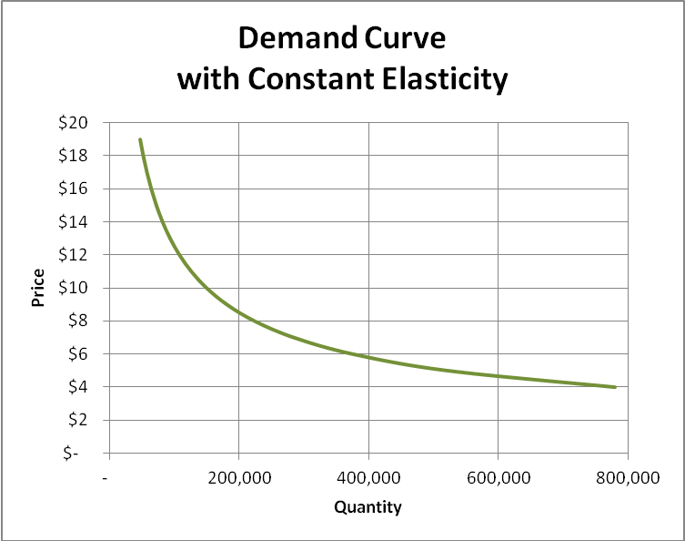
This is the demand function with a locally known elasticity. Qi and Pi are the known quantity sold at the known price. ε is the elasticity in demand around that price.
A plot this demand function can be found below given an elasticity of -1.8 (an average elasticity of demand for consumer products) around the price of $10 where 150,000 units are sold. Notice, lower prices are associated with higher sales volumes and higher prices are associated with lower sales volumes.
Step 4: Use the demand function to optimize the price against the firm’s profit function
From here, prices can be optimized against the firm’s profit equation. (Refer to Economic Price Optimization with Globally Linear Demand — Both Useful and Useless, for details.)
Start with the standard form of the firm’s profit equation
![]()
where π stand for the firm’s profit, Q stands for the quantity sold, P stands for the price of the product, V stands for the variable costs to make the product, and F stands for the firm’s fixed costs. There is nothing new in this equation. It is taught in freshman business classes.
As freshman calculus tells us, the first derivative of profits with respect to price equals zero where the profit function has reached a maximum for normal products. The price which delivers the maximum profits is clearly the optimal price.
In looking at the profit equation of the firm, we can see that a price change affects the firm’s profit directly through the variable P. We can also expect that a price change influences the quantity sold and so indirectly affects the firm’s profit through the variable Q. As for F and V, fixed costs and variable costs are constants with respect to a pure price change.
Taking the first derivative of the firm’s profit equation with respect to price and setting this equal to zero yields
![]()
where Q is defined above in relation to P through the elasticity and similarly the derivative of Q with respect to P is defined by the elasticity equation as
![]()
Inserting and simplifying, we find the optimal price for elasticity’s greater than one to be
![]()
We find the optimal price is dependent upon the variable costs and elasticity alone.
Notice fixed costs have no effect on the optimal price. Only the variable costs.
Step 5: Investigate the result
A numerical example will help us see what the resultant equations means.
Suppose a firm makes an item for $5, sells it for $ 10, and at $10, the firm sells 150,000 units. Furthermore, the firm has a fixed cost of $500,000. (V=$5, Pi=$ 10, Qi=150,000, F=$500,000)
Managers then go out and measure the elasticity of demand to optimize prices. Perhaps they use NPD data or they use their own transactional history. Either way, suppose they find the elasticity is about -1.8. I say about because they weren’t able to measure the elasticity exactly. Statistically, they may only know that it is -1.8 +/- 0.5. That is, they know it is around -1.8, but aren’t sure if it is higher or lower. It has a 95% probability of being somewhere between -2.3 (=-1.8 – 0.5) and -1.3 (=-1.8+0.5), and it is rather unlikely that it is really -1.8, but that is the manager’s best expectation.
(A note about statistics and measurements: the 95% confidence interval around a measurement is defined to be 1.96 standard deviations above and below the measurement.)
This is the nature of elasticity measurements. We rarely are able to measure elasticity precisely. We may able to narrow our uncertainty down to some range, but will never know it exactly. In studying years of transactional history on various specific products, I have seen many cases where the elasticity of demand was completely immeasurable and many cases where it could be measured to one significant digit only. Only in a relatively few unique cases, have I seen elasticity measured with any precision—that is, to two or more significant digits.
So what happens when we use our elasticity measurements to identify the “optimal” price? Well, since we can’t measure the elasticity exactly, we only know it falls within some range, we should similarly suspect we won’t find the optimal price exactly, only that it falls within some range. We may be satisfied with this since at least a range is better than nothing. So let’s find the range of prices associated with the expected range of elasticity found in the measurement. While we are at it, let’s also calculate the quantity sold and profit at each potential price.
We find the following for different expectations for price, quantity sold, and profits for the range of the elasticity of demand identified:
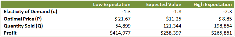
If you review the above table carefully, the challenge should become clear.
In this example, we stated managers were able to measure elasticity to be -1.8 +/- 0.5, which would be a very good measurement as measuring these things goes. With this measurement and level of precision, they would predict the optimal price to be $11.25 and should report that it could lie anywhere between $8.85 and $21.67. Now what should an executive do with this result?
Seriously, what would you do if you paid someone to tell you what price to use and they came back and said “I think $11.25 is best, but it could be anywhere between $9 and $21”? Would you say “well done” or would you toss them out as a waste of time and money? If the executive is managing thousands-to-millions of products and is able to identify the elasticity of demand for each product, even with some high level of uncertainty, relatively cheaply and time-efficiently, then, as a future argument will show, perhaps a pat on the back is deserved. But in most cases, they would be a tosser.
Now, if this approach isn’t good for pricing in most cases, what does it tell us? Examining the results of the numerical example reveals that a firm’s profits increase as the demand for their products become more inelastic. This in turn implies firms should focus on making the market demand for their offerings somewhat inelastic, and on finding customers whose demand for their offerings is somewhat inelastic. And how can firms do that? At this point, we have reentered the realm of market segmentation, branding, and value-based selling, the core of sales, marketing, and entrepreneurship.
4 Comments
About The Author

Tim, “Economic Price Optimization with Locally Measured
Elasticity of Demand — Unreliable”
I believe you are saying that using elasticity computed at one price to determining optimal prices is unreliable. This is certainly true because this method assumes that elasticity is constant across a range of prices. Using this method is equivalent to trying to find the maximum of a function by using a linear approximation to the function (more precisely, a linear approximation to the log of the function) in place of the real function.
a) A good solution to your problem is to allow elasticity to vary as a linear function over a range of prices. This method is equivalent to finding the maximum of a function using a quadratic approximation of the function, which generally works quite well.
Other limitations of using elasticity to optimize prices and solutions:
b) If variable costs are nonzero (which they almost always are), then optimizing revenue is the wrong problem to solve. We should be talking about maximizing contribution margin = revenue – variable costs.
c) Another complication is that sale of most products depends on pricing of similar products, including your products and competitors’ products. The solution is to use a multivariate price elasticity model that takes into account impact of prices for all the products on the sales of each product.
d) You can trust estimates of elasticity only if they pass tests of statistical significance: a t-test for elasticity estimates, and an F test for goodness of fit (r^2).
You can get price elasticity models in Excel that include all
enhancements listed above (a, b, c, d) and that are customizable to many
situations. For a price elasticity model for one product, see
http://bit.ly/sovhFn. For several products, see http://bit.ly/n0dVDT.
Further conditions must be met by market tests in order to
get solid estimates of price elasticities:
a) The market tests used to compute elasticity must meet some basic conditions. First, in the same price range, each test market should have the same price elasticity as every other test market. Secondly, each test market should not react to prices in other test markets. Thirdly, the temporary nature of test prices should have a negligible effect on buying behavior.
b) In some cases, winning in the long run strongly depends on being first (where market leadership has inertia) or on having the largest market share (due to large economies of scale), optimizing revenue or profit in the near term may be a very bad approach, from a strategic point of view. This
is where you need qualitative business strategy methods, or else a quantitative model that includes the long-term effects mentioned above.
Price elasticity provides a powerful and reliable way to set optimal prices, if these factors are taken into account.
How did you get the optimal quantities sold?
you plug the P identified back into the equation in Step 3
We work with adaptive/dynamic pricing in perishable inventory environments – elasticity is (generally) variable on a market, product and temporal basis
I would be very wary of any model that extrapolates a (potentially) stale or overly generalized elasticity
If the pricing strategy (or process) hinges on a “known” elasticity I would recommend carefully checking model sensitivity to a range of elasticities before embedding this approach
Consumers decide elasticity, and consumers are fickle creatures